
After the checks on the solar and magnetosphere parameters it is possible to start the reconstruction of the particle trajectory back in time. The motion equation is described by:
\begin{equation}
m\frac{d\vec{v}}{dt}=Zq\vec{v}\times\vec{B}
\end{equation}
where \(m\) and \(Z\) are the relativistic mass and the number of elementary charges of the particle, \(\vec{v}\) its velocity, \(q\) the electron charge and \(\vec{B}\) the magnetic field. The propagation equation remains unchanged when the charge sign and the velocity of the particle are simultaneously reversed. In fact, to trace a particle back in time we used the strategy to reconstruct the trajectory of a particle with opposite charge that is going in the opposite direction. The two trajectories, if there are not energy losses, should be the same. The first step is the evaluation of the particle velocity from its rigidity. With the total magnetic field (internal IGRF and external T96 or TS05 models), the Larmor radius is obtained:
\begin{equation}
r_L=\frac{m|\vec{v}|}{Zq|\vec{B}|}\ \ \ \Rightarrow\ \ \ \tau_g=\frac{2\pi r_L}{|\vec{v}|}.
\end{equation}
Integration step is small enough that linear approximation is possible and a value of 10\(^{-3}\) with respect to the gyroradius is the right compromise between precision and time computation. The differential equation (1) is solved step by step using the Runge Kutta method. This method gives the numerical solution for ordinary differential equation. Starting from a differential equation as:
\begin{equation}
\frac{dy}{dt}=f(t)
\end{equation}
with initial value \(y(t_0)=y_0\), we can build the solution \(y(t)\) moving from one point to the other using the Euler method as follows:
\begin{equation}
y_{n+1}=y_n+f(t_n,y_n)dt,
\end{equation}
but in our Runge Kutta method we calculate the solution using the Taylor's expansion of the function \(f(t)\) that for example at the second order is:
\begin{equation}
y_{n+1}=y_n+\frac{1}{2}h_n(f(t_n,y_n)+f(t_n+h_n,h_nf_n)),
\end{equation}
where \(f_n=f(t_n,y_n)\) and \(h_n=t_{n+1}-t_n\). Our code uses 6\(^{th}\) order version that is faster and more precise. The Earth magnetopause is calculated using Sibeck or Shue equations (Sibeck1991 and Shue1997). In the code we use the latest one (Shue). Particles are back-traced in time until they reach one of the two boundaries: the magnetopause (for primary CR) or again the detector altitude (secondary one). If the time of the reconstructed trajectory reached 10 seconds, we tag those particles as trapped, they did not reach the magnetopause and they did not recome back to the detector altitude. In the output of the code we have all the information related to the final point of the back-tracing, the total trajectory and a tag that indicates if the particle is coming from the boundary of the magnetosphere or if it is coming from an inner magnetosphere region.
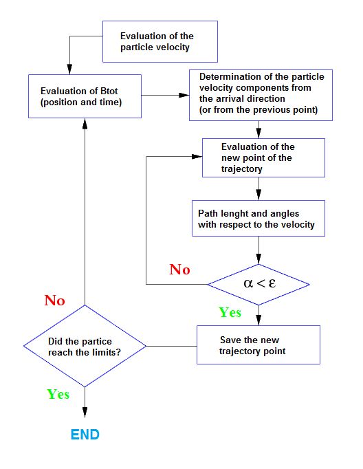
Figure 1: Sketch of the code.